Differentiate or integrate a function symbolically, then evaluate the result at a point or compute a definite integral over [a, b]. Free, instant, no sign-up.
Have feedback? Report bugs, suggest features, or share your thoughts — we read them all
What is a Derivative & Integral Calculator?
A derivative and integral calculator is a symbolic mathematics tool that computes derivatives (instantaneous rates of change) and antiderivatives or integrals (areas under curves) of mathematical functions. Unlike a plain numerical calculator that returns one number, a symbolic engine returns the exact algebraic answer — for instance, the derivative of x³ comes back as 3x², not a decimal at one specific point.
This calculator handles polynomials, trigonometric functions, exponentials, logarithms, and arbitrary compositions of them. It is built for students taking single-variable calculus, engineers checking by-hand work, and anyone who has to differentiate or integrate a function quickly without firing up Wolfram Mathematica or SymPy. The two operations — differentiation and integration — are inverses of each other, the central insight of the Fundamental Theorem of Calculus, which transformed mathematics in the late 17th century.
Derivatives
Definition
The derivative of a function f(x) is the instantaneous rate of change of f with respect to x. Geometrically, it is the slope of the tangent line to the curve y = f(x) at the point (x, f(x)). The rigorous definition is the limit of the slope of a secant line as the two endpoints come together:
f'(x) = lim[h→0] (f(x+h) − f(x)) / h
Common Derivative Rules
Power Rule: d/dx(xⁿ) = n·xⁿ⁻¹
Product Rule: d/dx(f·g) = f'·g + f·g'
Quotient Rule: d/dx(f/g) = (f'·g − f·g') / g²
Chain Rule: d/dx(f(g(x))) = f'(g(x))·g'(x)
Trigonometric Derivatives
d/dx(sin x) = cos x
d/dx(cos x) = −sin x
d/dx(tan x) = sec² x
Exponential & Logarithmic Derivatives
d/dx(eˣ) = eˣ
d/dx(ln x) = 1/x
d/dx(aˣ) = aˣ·ln a
Integrals
Definition
The integral of f(x) represents the signed area under the curve y = f(x). The indefinite integral (antiderivative) is the family of functions whose derivative is f(x); the definite integral computes a specific area between two limits:
∫f(x) dx = F(x) + C, where F'(x) = f(x)
Common Integral Rules
Power Rule: ∫xⁿ dx = xⁿ⁺¹/(n+1) + C (n ≠ −1)
Sum Rule: ∫(f + g) dx = ∫f dx + ∫g dx
Constant Multiple: ∫k·f dx = k·∫f dx
Trigonometric Integrals
∫sin x dx = −cos x + C
∫cos x dx = sin x + C
∫sec² x dx = tan x + C
Exponential & Logarithmic Integrals
∫eˣ dx = eˣ + C
∫(1/x) dx = ln|x| + C
∫aˣ dx = aˣ/ln(a) + C
Applications of Derivatives and Integrals
Derivatives and integrals appear in every quantitative discipline:
Physics: velocity is the derivative of position, acceleration the derivative of velocity; displacement is the integral of velocity
Economics: marginal cost and revenue are derivatives; total cost is the integral of marginal cost
Engineering: optimization problems set derivatives to zero; stress analysis integrates load functions; signal processing uses both
Biology: population growth rates and drug concentration models are differential equations
Computer graphics: Bézier and B-spline curves are defined by derivatives; physics-based animation integrates forces over time
Machine learning: gradient descent — the algorithm behind every neural network — works by computing derivatives of the loss function
Statistics: probability density functions are derivatives of cumulative distribution functions; expectation values are integrals
Always use explicit multiplication symbols (write 2*x, not 2x)
Use parentheses to make the order of operations clear
For trigonometric functions, the argument is in radians
Check your result by differentiating an integral (should get the original function)
Remember that indefinite integrals include an arbitrary constant C
Frequently Asked Questions
It says two things, both surprising. First (the differentiation part): if you define F(x) as the area under the graph of f from a fixed point a up to x, then F is differentiable and F'(x) = f(x). Building up area is exactly the inverse of taking instantaneous slope. Second (the evaluation part): to compute a definite integral ∫ᵃᵇ f(x) dx — the actual area — you find any antiderivative F of f and compute F(b) − F(a). You never have to evaluate the limit definition; you just look up an antiderivative in a table. This single theorem, discovered independently by Newton (1666) and Leibniz (1675), is what turned calculus from a curiosity into the engine of physics. Before it, computing the area under a parabola was an undergraduate-thesis-level result via the method of exhaustion; after it, every high schooler could do it in two lines. The theorem is also why physicists feel free to write things like 'work = ∫ F·dx': they know that integrating force with respect to position is the same as undoing differentiation, which connects directly to potential energy.
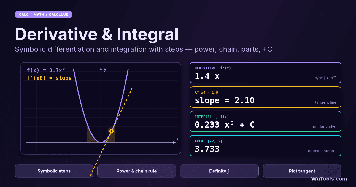
After you compute a symbolic answer, this calculator can plug in a number for you. For a derivative (or nth derivative), type the value into the 'Evaluate at' field — for example enter 2 to get the slope f'(2) as an actual number, not a formula. The tool substitutes that value into the simplified derivative using the built-in math engine and prints f'(2) = N below the result. This is exactly what an engineer or analyst usually needs: the formula f'(x) = 3x² is only the first step; the number f'(2) = 12 is the marginal rate, the tangent slope, or the instantaneous velocity at that point. If the expression contains symbolic constants other than your variable (say a parameter a), evaluation will fail because the value isn't fully numeric — substitute or remove those symbols first. Leave the field blank to get the symbolic answer only.
Switch the operation to Integral, enter your function, then fill in the 'From' and 'To' bounds that appear. The tool first finds an antiderivative F(x) symbolically, then applies the Fundamental Theorem of Calculus: the definite integral over [a, b] equals F(b) − F(a). It drops the '+ C' (which always cancels in a definite integral) and prints the numeric area, e.g. ∫[0, 2] x^2 dx = 2.6667. Leave both bounds empty to get only the indefinite integral (antiderivative + C). Two caveats: the integration engine handles elementary base rules — powers x^n, sums, constant multiples, sin(x), cos(x), e^x, a^x and 1/x — but not integration by parts or substitution at runtime, so a function like sin(2*x) or x*e^x will report that it cannot be integrated. And the bounds must be plain numbers; symbolic limits are not supported.
Apply the limit definition: f'(x) = lim[h→0] (f(x+h) − f(x))/h. With f(x) = x², the numerator becomes (x+h)² − x² = x² + 2xh + h² − x² = 2xh + h². Divide by h: 2x + h. Now take the limit as h approaches zero: the h-term vanishes and you're left with 2x. So f'(x) = 2x. Geometrically, this matches: at x = 0 the curve is flat (slope 0 = 2·0), at x = 1 the slope is 2 (the tangent rises one unit for every half-unit run), at x = −3 the slope is −6 (steep downward). The power rule d/dx(xⁿ) = n·xⁿ⁻¹ generalises this exact same argument: for x³ you get 3x² because the cubic expansion has a leading 3x²h term that survives; for x⁴ you get 4x³; and so on. The pattern works for any real exponent — fractional, negative, irrational — though the proof for non-integer exponents needs the chain rule and the logarithmic derivative. This is why the power rule is the first thing every calculus student memorises: it handles polynomials and most algebraic expressions instantly.
Use the chain rule whenever your function is a composition of two functions — an 'outside' applied to an 'inside'. For example, sin(x²) is the sine of x squared; cos(3x + 1) is cosine of a linear expression; e^(−x²) is exp applied to −x². The rule says: differentiate the outside function evaluated at the inside, then multiply by the derivative of the inside. So d/dx[sin(x²)] = cos(x²) · 2x. For e^(−x²), the outside is exp (derivative also exp), the inside is −x² (derivative −2x), giving −2x · e^(−x²). Identify compositions by asking 'if x were a single variable u, what would I do?' — then apply the answer to u = g(x) and multiply by g'(x). The chain rule is the most-used rule in calculus because almost every interesting function is a composition: ln(sin x), (3x+5)^7, √(x²+1), and so on. It is also what makes neural networks trainable — backpropagation is just the chain rule applied repeatedly across layers.
Because two functions that differ by a constant have the same derivative. If F(x) is an antiderivative of f(x), then so is F(x) + 7, F(x) + π, or F(x) − 1000 — they all differentiate back to f(x), because the derivative of any constant is zero. So when you compute ∫f(x) dx, the answer isn't a single function but a whole family of functions, each shifted vertically from the others. We write '+ C' to acknowledge that any constant could be there. This isn't pedantry — it matters in physics. If you integrate acceleration to find velocity, the +C is the initial velocity, which you can't recover from acceleration alone. If you integrate velocity to find position, the +C is the initial position. In a definite integral ∫ᵃᵇ f(x) dx, the +C cancels because you compute F(b) + C − (F(a) + C), which is just F(b) − F(a). So definite integrals don't need +C, but indefinite integrals always do. Forgetting +C on an exam loses you a point; forgetting initial conditions on a physics problem loses you the answer.
Symbolic integration produces an exact formula: ∫x² dx = x³/3 + C, ∫sin(x) dx = −cos(x) + C, ∫1/x dx = ln|x| + C. The answer is an algebraic expression you can manipulate further. This calculator does symbolic integration. Numerical integration produces a number that approximates a definite integral: ∫₀¹ e^(−x²) dx ≈ 0.7468. It doesn't tell you what the antiderivative looks like, but it gives you the area. Most real-world integrals are computed numerically using methods like Simpson's rule, the trapezoidal rule, or Gaussian quadrature — because real-world integrands rarely have nice closed-form antiderivatives. SciPy's scipy.integrate.quad, MATLAB's integral(), and Python's standard library all use sophisticated numerical schemes. Choose symbolic when you need the formula (taking further derivatives, solving differential equations algebraically, simplifying); choose numerical when you only need a definite value to specified precision and the integrand might not have an elementary antiderivative.
These are the two inverses of the differentiation rules — the substitution rule inverts the chain rule, and integration by parts inverts the product rule. Substitution (u-substitution): when you spot a function and its derivative both present in the integrand, set u equal to the inner function and replace dx with du/g'(x). Example: ∫ 2x·cos(x²) dx — let u = x², du = 2x dx, integral becomes ∫cos(u) du = sin(u) + C = sin(x²) + C. Integration by parts: when the integrand is a product, ∫u dv = uv − ∫v du. Pick u so that u' is simpler than u, and dv so that v is easy to find. Example: ∫x·eˣ dx — let u = x (so du = dx) and dv = eˣ dx (so v = eˣ), giving x·eˣ − ∫eˣ dx = x·eˣ − eˣ + C. The mnemonic LIATE (Logarithm, Inverse trig, Algebraic, Trig, Exponential) helps pick u — try the type that appears earliest in the list. These two tricks plus partial fractions handle the vast majority of integrals you encounter in a calculus course.
Because the family of elementary functions — polynomials, exponentials, logarithms, trigonometric functions, and their inverses, combined by addition, multiplication, division, and composition — is closed under differentiation but NOT closed under integration. The classic counter-example is ∫e^(−x²) dx, the integral that gives the normal distribution. Despite the integrand being a simple-looking composition of exp and a quadratic, there is no finite combination of elementary functions whose derivative is e^(−x²). Joseph Liouville proved this in 1835: he showed that if such an antiderivative existed, it would have to be of a specific algebraic form, and then derived a contradiction. The same fate befalls ∫(sin x)/x dx, ∫√(1 + x³) dx, ∫1/ln(x) dx and many others. These integrals do have antiderivatives — they exist as functions — they just can't be written using the elementary toolkit. Mathematicians have invented special-function names: the integral of e^(−x²) is called the error function erf(x), the integral of (sin x)/x is called Si(x), and so on. So 'can't be integrated' doesn't mean 'impossible' — it means 'no elementary formula exists, so we either give it a new name or compute it numerically'.
Every modern machine learning model is trained by gradient descent, which is calculus repeated millions of times. You have a loss function L(θ) — a single number measuring how badly the model's predictions miss the training data, as a function of the model parameters θ (which can be billions of numbers in a large language model). You want to find θ that minimises L. Calculus says: at a minimum, the gradient ∇L is zero. Gradient descent uses the chain rule to compute ∂L/∂θᵢ for every parameter θᵢ, then takes a small step in the negative-gradient direction: θ ← θ − α·∇L. Repeat thousands of times. The chain rule is essential because L is a deep composition: input goes through layer 1, then layer 2, ..., then the loss is computed. Backpropagation — invented by Linnainmaa (1970), rediscovered and popularised by Rumelhart, Hinton and Williams (1986) — is the chain rule applied backwards through the layers, efficiently computing all the partial derivatives in one pass. Without symbolic differentiation (or its modern cousin, automatic differentiation as in PyTorch and TensorFlow), neural networks would be untrainable. So when ChatGPT generates a sentence, calculus is doing the heavy lifting underneath.